


Next: 6 伝達関数 1次の場合
Up: オーディオのための交流理論入門
Previous: 4 複数の素子を組み合わせた場合
前節で使ったベクトル図では,ベクトルの長さが正弦波の振幅を,
方向が正弦波の初期位相を表していました.
ベクトルの長さは計算で求められましたが,
方向は図の上で表していました.
特に,コンデンサやコイルによって,位相が 90o ずれることを,
数式としてではなく,図で表していました.
位相を変化させることは,数式でも表せます.
図31のように,
振幅が r,初期位相が  の正弦波の位相を
  だけ進めることを
考えましょう.
だけ進めることを
考えましょう.
図 31:
ベクトルの回転
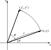 |
図より,
| x |
= |
r cos |
(58) |
| y |
= |
r sin |
(59) |
| x' |
= |
r cos( +  ) ) |
(60) |
| y' |
= |
r sin( + ) |
(61) |
加法定理を使うと,
| x' |
= |
r cos( + ) |
|
| |
= |
r coscos - r sinsin |
|
| |
= |
x cos - y sin |
(62) |
| y' |
= |
r sin( + ) |
|
| |
= |
r cossin + r sincos |
|
| |
= |
x sin + y cos |
(63) |
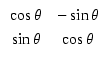
これを行列を使って表すと,
となります.
一応,数式で表せたのですが,行列を使わねばなりません.
これまで,xy 平面を使ってきましたが,
y 軸を虚数とすることで,このめんどうなベクトルの回転の計算が,
単純な掛け算になってしまいます.
複素数を使うことによって,たとえば電圧と電流の関係を,その大きさだけでなく,
位相を含めてオームの法則と同様な式で表すことができるようになります.
複素数(complex number)は,
実数 a と虚数 jb3 を組み合わせた数です.
すなわち,
|
Z = a + jb (直角座標表示またはガウス平面表示)
|
(65) |
です.
j は,虚数単位で,
です.
複素数は,横軸に実数軸,縦軸に虚数軸をとった複素平面上の点を表していると考えられます.
与えられた Z から,実数部 a および虚数部 b を取り出す操作を,次の式で表します.
| a |
= |
 Z Z |
(67) |
| b |
= |
 Z Z |
(68) |
図 32:
複素数の表示
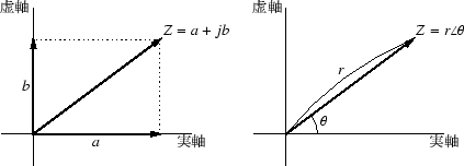 |
また,複素平面上の点は,原点 O からの距離 r と,実数軸からの角度 で表すこともできます.
Z = r (ベクトル表示) (ベクトル表示)
|
(69) |
r を Z の大きさまたは絶対値(absolute value)といい,
を Z の偏角(angle)といいます.
これらは,それぞれ正弦波の振幅,(初期)位相です.
与えられた Z から大きさや偏角を取り出す操作を,次の式で表します.
| r |
= |
| Z| |
(70) |
|
= |
arg Z |
(71) |
複素数の直角座標表示とベクトル表示を比較すると,
次の関係がわかります.
| r |
= |
 |
(72) |
| tan |
= |
 |
(73) |
| a |
= |
r cos |
(74) |
| b |
= |
r sin |
(75) |
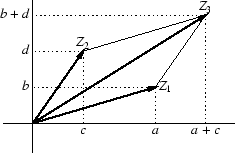
Z1 = a + jb と Z2 = c + jd を加えると,
|
Z3 = Z1 + Z2 = (a + jb) + (c + jd )= (a + c) + j(b + d )
|
(76) |
図 33:
複素数の加算
 |
Z1 = a + jb と Z2 = c + jd を掛け合わせると,
| Z3 |
= |
Z1Z2 |
|
| |
= |
(a + jb)(c + jd ) |
|
| |
= |
ac + jad + jbc + j2bd |
|
| |
= |
(ac - bd )+ j(ad + bc) |
|
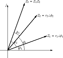
Z1, Z2, Z3 をベクトル表示にすると,
| r1 |
= |
| Z1| = |
|
 |
= |
arg Z1 = tan-1 |
|
| r2 |
= |
| Z2| =  |
|
 |
= |
arg Z2 = tan-1 |
|
| r3 |
= |
| Z3| = 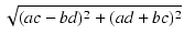 |
|
| |
= |
 |
|
| |
= |
 |
|
| |
= |
 |
|
| |
= |
r1r2 |
|
 |
= |
arg Z3 = tan-1 |
|
| |
= |
tan-1 |
|
| |
= |
tan-1 |
|
| |
= |
tan-1 |
|
| |
= |
tan-1tan( + ) |
|
| |
= |
+ |
|
となるので,
複素数の乗算は,大きさを掛け合わせ,偏角を加えることになります.
すなわち,
|
Z3 = Z1Z2 = (r1)(r2) = r1r2( + )
|
(77) |
図 34:
複素数の乗算
 |
割り算の場合は,
| Z3 |
= |
 |
|
| |
= |
 |
|
| |
= |
.  |
|
| |
= |
 |
|
| |
= |
 + j + j |
|
| r3 |
= |
 |
|
| |
= |
 |
|
| |
= |
 |
|
| |
= |
 |
|
| |
= |
 |
|
| |
= |
 |
|
|
= |
tan-1 |
|
| |
= |
tan-1 |
|
| |
= |
tan-1 |
|
| |
= |
tan-1 |
|
| |
= |
tan-1 |
|
| |
= |
tan-1tan( - ) |
|
| |
= |
- |
|
これより,複素数の割り算は,大きさを割り算し,偏角は引き算したものになります.
すなわち,
まとめると,
| | Z1 . Z2| |
= |
| Z1| . | Z2| |
(79) |
| arg(Z1 . Z2) |
= |
arg Z1 + arg Z2 |
(80) |
  |
= |
 |
(81) |
arg  |
= |
arg Z1 - arg Z2 |
(82) |
となります.
これまでと同じように,原点の周りを長さが Vm の棒が反時計方向に回っているとします.
時刻 0 における棒の大きさと向きは,
Vm であり,
時刻 t における棒の向きは,その位相をさらに
であり,
時刻 t における棒の向きは,その位相をさらに  t 進めたものですから,
Vm( t + ) = (Vm) . (1t) t + ) = (Vm) . (1t)
|
(83) |
で表せます.
正弦波の瞬時値は,棒の先の y 軸方向の高さなので,
複素数平面では,虚数成分を取り出すことになり,
|
v(t) = {(Vm) . (1t)}
|
(84) |
で表せます.
このように,振幅と初期位相がわかれば,任意の時刻における瞬時値を求めることができるので,
振幅と初期位相によるベクトル表示をもって,正弦波を表すことにします4.
正弦波の振幅は,複素数  の絶対値になります
.
初期位相は,複素数 の偏角になります.
の絶対値になります
.
初期位相は,複素数 の偏角になります.
位相を 進めることは,
1 を掛けることになります.
特に,位相を 90o 進めることは,
|
190o = cos 90o + j sin 90o = 0 + 1j = j
|
(88) |
を掛けることになります.
位相を 90o 遅らせることは,
|
1(- 90o) = cos(- 90o) + j sin(- 90o) = 0 - 1j = - j
|
(89) |
を掛けることになります.
より,
位相を 90o 遅らせることは,j で割るといってもよいでしょう.
複素数の割り算は,位相を引くことであることを思い出してください.
コンデンサに掛かっている電圧と電流の関係は,式(15)より,
| vC |
= |
Vmsin(t) |
(91) |
| iC |
= |
VmC cos(t) = VmC sin(t +  /2) /2) |
(92) |
これを複素数のベクトル表示で表すと,
 |
= |
Vm 0 |
(93) |
 |
= |
VmC(/2) |
(94) |
インピーダンスを複素数で表すと,
1(-  /2) = 1/j なので,
 = = 
|
(96) |
となります.
コイルに掛かっている電圧と電流の関係は,式(17)より,
| vL |
= |
Vmsin(t) |
(97) |
| iL |
= |
-  cos(t) = sin(t - /2) cos(t) = sin(t - /2) |
(98) |
これを複素数のベクトル表示で表すと,
 |
= |
Vm 0 |
(99) |
 |
= |
(- /2) |
(100) |
インピーダンスを複素数で表すと,
1(/2) = j なので,
 = jL = jL
|
(102) |
となります.
コンデンサやコイルのインピーダンスを複素数で表すと,
位相が回転する情報も含めて,オームの法則と同様に扱うことができます.
図16のローパスフィルタも,分圧回路と見なして計算できます.
伝達関数
 (j) は,入力に対する出力で定義され,
となります.
分母に虚数単位が入っていると不便なので,有理化しておきましょう.
ゲインは,この伝達関数の絶対値に,(入力に対する出力の)位相は伝達関数の偏角になります.
具体的に計算してみましょう.
複素数の絶対値は,
| Z| =  ですから,
ですから,
A = 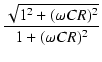 = = 
|
(107) |
となります.
位相は,
arg (j) (j) |
= |
tan-1 |
|
| |
= |
tan-1 |
|
| |
= |
tan-1(- CR) |
(108) |
となります.
Rでグラフを描いてみます.
function ()
{
    R <- 15.9e3         # 抵抗値
    C <- 0.01e-6        # 容量

    f <- dec(10, 100e3, 30)         # 周波数
    w <- 2 * pi * f                 # 角周波数
    A <- 1/sqrt(1 + w * C * R)      # ゲイン
    phi <- atan(-w * C * R)         # 位相

    par(mfrow=c(2, 1))
    semilogplot(f, dB(A), type="l", col="red",
        xlab="Frequency (Hz)", ylab="Gain (dB)")
    semilogplot(f, phi*180/pi, type="l", col="red",
        xlab="Frequency (Hz)", ylab="Phase (deg)")
}
Rの場合は,複素数をそのまま扱えますから,
次のようにすることもできます.
function ()
{
    R <- 15.9e3         # 抵抗値
    C <- 0.01e-6        # 容量

    f <- dec(10, 100e3, 30)         # 周波数
    w <- 2 * pi * f                 # 角周波数
    j <- 0+1i                       # 虚数単位
    T <- 1/(1 + j * w * C * R)      # 複素数による伝達関数

    par(mfrow=c(2, 1))
    semilogplot(f, dB(T), type="l", col="red",
        xlab="Frequency (Hz)", ylab="Gain (dB)")
    semilogplot(f, Arg(T)*180/pi, type="l", col="red",
        xlab="Frequency (Hz)", ylab="Phase (deg)")      # Arg は偏角を得る関数
}
式(104)を複素数のまま計算し,
abs() を使えば複素数の絶対値が得られ,
Arg() を使えば複素数の偏角が求められます.
dB() の中には,abs() が入っていますので,
そのまま dB(T) とすればゲインのデシベル値が求められます.
Rの虚数の表現は,a+bi ですが,結合がそれほど強くないので,
式の中で使う時は (a+bi) のようにかっこで囲んだほうが良いでしょう.
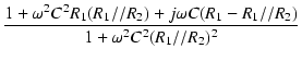
図29の回路の伝達関数を求めます.
伝達関数は,
| T(j) |
= |
 |
|
| |
= |
 |
|
| |
= |
 |
|
| |
= |
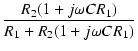 |
|
| |
= |
 . .  |
|
| |
= |
.  |
(109) |
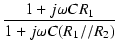
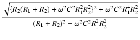
分母を有理化すると,
| T(j) |
= |
. .  |
|
| |
= |
.  |
|
| |
= |
. 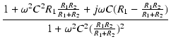 |
|
| |
= |
R2 . 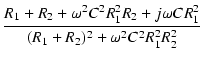 |
|
| |
= |
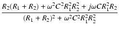 |
(110) |
ゲインは,
| | T(j)| |
= |
 |
|
| |
= |
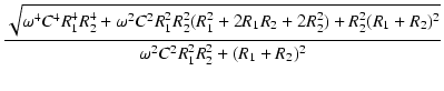 |
|
| |
= |
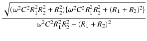 |
|
| |
= |
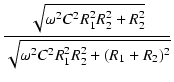 |
|
| |
= |
. 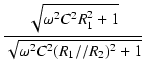 |
(111) |
となり,式(57)と一致しました.
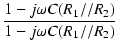
位相は,
| arg T(j) |
= |
tan-1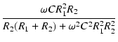 |
|
| |
= |
tan-1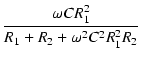 |
(112) |
となります.
Rで周波数特性を描いてみると,
function ()
{
    R1 <- 1e3
    R2 <- 100
    C <- 1000e-12

    f <- dec(1e3, 10e6, 30)
    w <- 2 * pi * f
    A <- R2 / (R1 + R2) *
        sqrt(w^2*C^2*R1^2 + 1) / sqrt(w^2*C^2*(R1 %p% R2)^2 + 1)
    phi <- atan((w*C*R1^2)/(R1 + R2 + w^2*C^2*R1^2*R2))

    par(mfrow=c(2, 1))
    semilogplot(f, dB(A), type="l", col="red",
        xlab="Frequency (Hz)", ylab="Gain (dB)")
    semilogplot(f, phi*180/pi, type="l", col="red",
        xlab="Frequency (Hz)", ylab="Phase (deg)")
}
%p% は抵抗,コイルの並列合成値を求める演算子です(コンデンサの場合は直列合成値になる).
このように,Rでは演算子も自分で定義することができます.
便利でしょう?
このプログラムのように,複素数を使わずに計算しようとすると,
人間が有理化してやらねばならず,計算が大変です.
複素数のまま計算すると,次のようになります.
function ()
{
    R1 <- 1e3
    R2 <- 100
    C <- 1000e-12

    j <- 0+1i
    f <- dec(1e3, 10e6, 30)
    w <- 2 * pi * f
    T <- R2 / (R1 + R2) * (1 + j*w*C*R1) / (1 + j*w*C*(R1 %p% R2))

    par(mfrow=c(2, 1))
    semilogplot(f, dB(T), type="l", col="red",
        xlab="Frequency (Hz)", ylab="Gain (dB)")
    semilogplot(f, Arg(T)*180/pi, type="l", col="red",
        xlab="Frequency (Hz)", ylab="Phase (deg)")
}
さらに,伝達関数を明に求めなくても計算できます.
function ()
{
    R1 <- 1e3
    R2 <- 100
    C <- 1000e-12

    j <- 0+1i
    f <- dec(1e3, 10e6, 30)
    w <- 2 * pi * f
    ZC <- 1/(j * w * C)     # Cの複素インピーダンス
    Z1 <- R1 %p% ZC         # R1 と C を並列にした複素インピーダンス
    T <- R2 / (Z1 + R2)     # 分圧

    par(mfrow=c(2, 1))
    semilogplot(f, dB(T), type="l", col="red",
        xlab="Frequency (Hz)", ylab="Gain (dB)")
    semilogplot(f, Arg(T)*180/pi, type="l", col="red",
        xlab="Frequency (Hz)", ylab="Phase (deg)")
}
こうすれば,人間が行う計算はほとんどなくなりますが,
どこにポールやゼロがあるかわかりませんので,
できれば伝達関数を求めておくのがよいでしょう.
複素数には,指数関数表示というもう一つの表現方法があります.
指数関数表示を使うと,複素数の積がもっと簡単に計算できます.
無限回微分可能な関数 f (x) は,
次の形のべき級数で表せます.
| f (x) |
= |
  (x - a)n (x - a)n |
(113) |
| |
= |
f (a) + f(1)(a)(x - a) +  (x - a)2 + (x - a)2 +  (x - a)3 + (x - a)3 +  (x - a)4 + ... (x - a)4 + ... |
(114) |
これをテイラー展開といいます.
ここで,
f(n)(x) は,f (x) を n 回微分したものです.
特に,a = 0 のとき,
| f (x) |
= |
 xn xn |
(115) |
| |
= |
f (0) + f(1)(0)x +  x2 + x2 +  x3 + x3 +  x4 + ... x4 + ... |
(116) |
となり,マクローリン展開といいます.
指数関数 ex は,何回微分しても ex であり,e0 = 1 ですから,
ex = 1 + x +  + +  + +  + +  + +  + +  + ... + ...
|
(117) |
となります.
この式の x のかわりに jx を代入すると,
| ejx |
= |
1 + jx +  + +  + +  + +  + +  + +  + ... + ... |
|
| |
= |
1 + jx - -  + + + +  - - - -  + ... + ... |
(118) |
となります.
sine関数を微分すると,次のようになります.
 |
= |
cos x |
(119) |
 |
= |
-sin x |
(120) |
 |
= |
-cos x |
(121) |
 |
= |
sin x |
(122) |
4回微分すると元に戻ります.
これから,sin x をマクローリン展開すると,
| sin x |
= |
sin 0 + x cos 0 - sin 0 - cos 0 + sin 0 + ... |
|
| |
= |
x - + - + ... |
(123) |
となり,
cos x をマクローリン展開すると,
| cos x |
= |
cos 0 - x sin 0 - cos 0 + sin 0 + cos 0 + ... |
|
| |
= |
1 - + - + ... |
(124) |
となります.
これら2つの式から,
| cos x + j sin x |
= |
1 - + - + ... + jx - + - + ... |
|
| |
= |
1 + jx - - + + - - + ... |
(125) |
となって,式(118)と一致します.
すなわち,
|
cos x + j sin x = ejx
|
(126) |
であり,これはオイラーの公式とよばれるものです.
sine関数は4回微分すると元に戻り,
j は4乗すると元に戻るという性質を考えると,
複素数と三角関数は密接な関係にあることが理解できます.
この式の x に を代入し,両辺を r 倍してやると,
r cos + jr sin = rej
|
(127) |
となり,これは図32の複素数を表しているといえます.
つまり,
|
Z = r = rej = r cos + jr sin
|
(128) |
で,これらは同じ複素数を別の形で表したものです.
この指数形式を使うと,複素数の乗算がとても簡単にできます.
r1ej . r2ej . r2ej = r1r2ejej = r1r2ej(+) = r1r2ejej = r1r2ej(+)
|
(129) |
正弦波の瞬時値は,
で表せます.
Next: 6 伝達関数 1次の場合
Up: オーディオのための交流理論入門
Previous: 4 複数の素子を組み合わせた場合
Ayumi Nakabayashi
平成19年12月8日
 =
=  =
= 


